Nancy Martel
Université du Québec à Rimouski
Rimouski, QC.
Studies on river confluences have highlighted the complex relationships between flow structure, sediment transport and bedforms development (Rice et al.., 2008). The shear layer between the two rivers is particularly dynamic and complex, with vertical vortices combined to streamwise secondary flow associated with the tributary curvature. The visualization of turbulent structures in the shear layer is possible by the injection of tracers or when sediment load allows a different turbidity flow (Biron et al, 1993; 1996; De Serres et al, 1999; Sukhodolov and Rhoads, 2004). The spatial location of the shear layer will depend on the momentum flux ratio (Mr) between the tributary and main channel, where momentum flux is the product of mass density, velocity and discharge rate.
In cold regions, where ice cover occurs for most of the winter period, flow structure is also likely to be affected by the roughness effect of the ice cover. The ice cover causes flow resistance that produces a second boundary layer changing the structure and turbulence of river flows. The expected velocity profile under an ice cover is characterized by a parabolic shape in which the maximum velocity is moved toward the center of the water column with increasing roughness (Crance and Frothingham, 2008). It has been documented that this shift in the location of the maximum velocity modifies the three-dimensional flow field in meander loops with an ice cover. Studies have highlighted the presence of superimposed helical cells with a reverse rotation direction (Urroz and Ettema 1994; Demers et al., 2011)
Although the flow structure at river confluence is relatively well documented and the general effect of an ice cover on the flow is known, the relationship between the flow structure and ice cover at confluences have yet to be explored. The aim of this study is to characterize and compare the flow structure at a medium sized confluence with and without an ice cover.
The confluence of the Mitis-Neigette River is located in Sainte-Angèle-de-Mérici in Eastern Québec (Figure 1). The confluence was selected because a thick ice cover is present for most of the winter allowing for safe field work. But winter field work remains challenging!
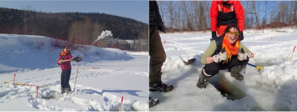
The winter field campaign took place in late February, early March, 2015. During this period, the outdoor maximum temperature ranged between -9°C and -22°C, which created difficulties for instrument batteries. Measurements of the ice-cover thickness, ice type and under-ice cover roughness were taken (Figure 3). Under-ice cover roughness measurements were obtained for 2m2 ice blocks by flipping them over to expose the undercover to produce a high resolution digital surface using a terrestrial LiDAR (Leica Scanstation, Figure 4). Bed topography was measured by ground-penetrating radar (Figure 5).
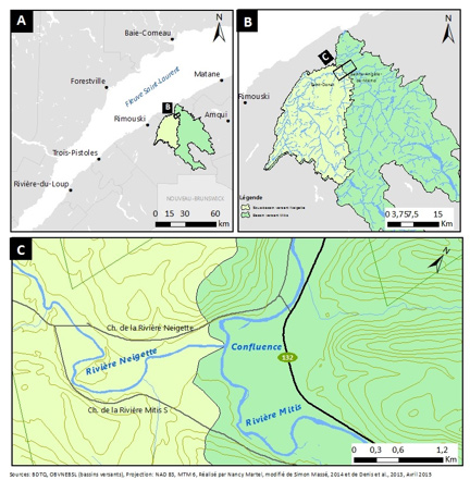
Figure 1 Location of the Mitis-Neigette confluence.

Figure 2 Vertical picture taken with a drone in winter and the location of the velocity profiles sampled with the ADV and ADCP.
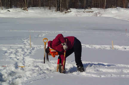
Figure 3 Measurements of ice- cover thickness
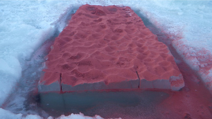
Figure 4 Roughness under the ice cover
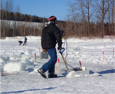
Figure 5 Measurements of bed topography with a ground-penetrating radar
As the focus of this study is flow dynamics of the shear layer, velocity profiles were collected with an acoustic Doppler current profiler (ADCP) to reconstruct the three-dimensional flow structure with 15 min-long velocity profiles collected at a sampling frequency of 1Hz (Figure 6). Vertical profiles were also measured using an acoustic Doppler velocimeter (ADV) to characterize the size and frequency of turbulent flow structures within the shear layer (Figure 7). Between 20 and 30 velocity profiles were collected for 3 minutes at a sampling frequency of 25 Hz with the ADV. This required the use of a tripod, anchored in the ice cover with ice screws, to limit problems of vibration that could contaminate the ADV signal (Figure 8).
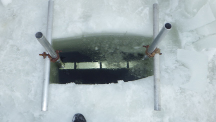
Figure 6 Field setup for velocity measurements with an ADCP
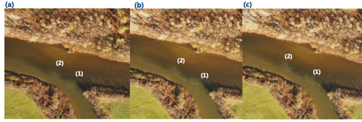
Figure 7 Observation of spatio-temporal evolution of vortical flow structures in the shear layer. Photos taken from a drone at time a) 3 sec, b) 9 sec and c) 15 sec
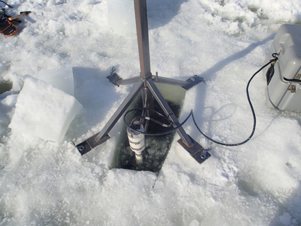
Figure 8 Tripod used to measure velocity with an ADV
he main challenges of this winter campaign pertain to velocity profile measurements as the cold affected both the instrumentation and field assistants. For example, the ADV tripod had sliding parts that froze during the night and that we had to unfreeze in the morning. The best technique was to insert it into the water, which was warmer than air, and wait about 30 minutes and then force a little sliding of the pole. This took 3 or 4 people. Likewise, using a chain saw to cut the ice cover was not simple. Because the winter 2015 was particularly cold, the ice cover was in some places thicker than the length of the blade (36-inch long) (Figure 9). On many occasions water ended up in the engine and we had to dry it using the generator’s exhaust pipe (Figure 10). We also lost a Toughbook computer in this adventure, as while during the installation of the ADCP the chain saw to cut the ice came a little bit too to close to the computer which received a massive waterjet (Figure 11). The computer did not survive….
In addition to the field measurement challenges, it was also difficult to locate the shear layer, which in summer condition is very obvious because of a turbidity difference between the two channels. On the plus side, taking measurements from the ice cover allows a great deal of flexibility as all areas of the confluence zone are accessible.
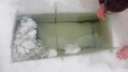
Figure 9 When ice thickness was larger than the blade length (36 inches), holes had to be cut in two steps

Figure 10 System used to dry the chain saw engine using the generator exhaust pipe
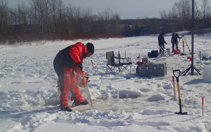
Figure 11 When we use chain saw for cut the ice cover a waterjet was produced
Overall, despite the challenges, we were able to collect great data which are currently being analyzed. With plenty of warm liquid and home-made brownies, winter field work can actually be fun!